The content of this tutorial is mainly based on the excellent books “Hands-on machine learning with scikit-learn, keras and tensorflow” from Aurélien Géron (2019) and “Tidy Modeling with R” from Max Kuhn and Julia Silge (2021)
In this tutorial, we’ll build the following classification models using the tidymodels framework, which is a collection of R packages for modeling and machine learning using tidyverse principles:
- Logistic Regression
- Random Forest,
- XGBoost (extreme gradient boosted trees),
- K-nearest neighbor
- Neural network
Note that due to performance reasons, I only show the code for the neural net but don’t actually run it.
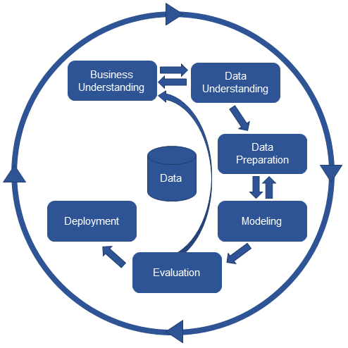
Furthermore, we follow this data science lifecycle process:
Business understanding
In business understanding, you:
- Define your (business) goal
- Frame the problem (regression, classification,…)
- Choose a performance measure
- Show the data processing components
First of all, we take a look at the big picture and define the objective of our data science project in business terms.
In our example, the goal is to build a classification model to predict the type of median housing prices in districts in California. In particular, the model should learn from California census data and be able to predict wether the median house price in a district (population of 600 to 3000 people) is below or above a certain threshold, given some predictor variables. Hence, we face a supervised learning situation and should use a classification model to predict the categorical outcomes (below or above the preice). Furthermore, we use the F1-Score as a performance measure for our classification problem.
Note that in our classification example we again use the dataset from the previous regession tutorial. Therefore, we first need to create our categorical dependent variable from the numeric variable median house value. We will do this in the phase data understanding during the creation of new variables. Afterwards, we will remove the numeric variable median house value from our data.
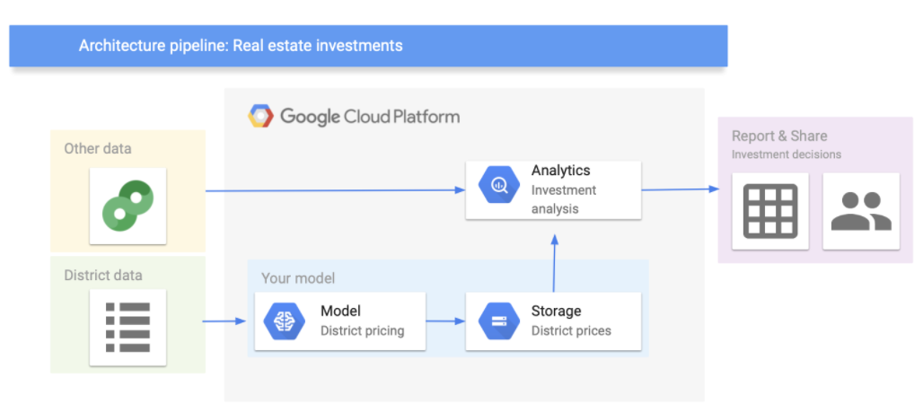
Let’s assume that the model’s output will be fed to another analytics system, along with other data. This downstream system will determine whether it is worth investing in a given area or not. The data processing components (also called data pipeline) are shown in the figure below (you can use Google’s architectural templates to draw a data pipeline).
Data understanding
In Data Understanding, you:
- Import data
- Clean data
- Format data properly
- Create new variables
- Get an overview about the complete data
- Split data into training and test set using stratified sampling
- Discover and visualize the training data to gain insights
Setup
If you like to install all packages at once, use the code below.
install.packages(c("tidyverse", "skimr", "GGally", "ggmap", "visdat", "corrr", "ggsignif", "gt", "vip", "themis", "purrr", "tidyr", "tidymodels", "keras", "ranger", "xgboost", "kknn")) library(tidyverse)
library(skimr)
library(GGally)
library(ggmap)
library(visdat)
library(corrr)
library(ggsignif)
library(gt)
library(vip)
library(themis)
library(purrr)
library(tidyr)
library(tidymodels)
library(keras)
library(ranger)
library(xgboost)
library(kknn)Import Data
First of all, let’s import the data:
LINK <- "https://raw.githubusercontent.com/kirenz/datasets/master/housing_unclean.csv"
housing_df <- read_csv(LINK)
Clean data
To get a first impression of the data we take a look at the top 4 rows:
housing_df |>
  slice_head(n = 4) |>
gt() # print output using gt| longitude | latitude | housing_median_age | total_rooms | total_bedrooms | population | households | median_income | median_house_value | ocean_proximity |
|---|---|---|---|---|---|---|---|---|---|
| -122.23 | 37.88 | 41.0years | 880 | 129 | 322 | 126 | 8.3252 | 452600.0$ | NEAR BAY |
| -122.22 | 37.86 | 21.0 | 7099 | 1106 | 2401 | 1138 | 8.3014 | 358500.0 | NEAR BAY |
| -122.24 | 37.85 | 52.0 | 1467 | 190 | 496 | 177 | 7.2574 | 352100.0 | NEAR BAY |
| -122.25 | 37.85 | 52.0 | 1274 | 235 | 558 | 219 | 5.6431 | 341300.0 | NEAR BAY |
Notice the values in the first row of the variables housing_median_ageand median_house_value. We need to remove the strings “years” and “$”. Therefore, we use the function str_remove_all from the stringr package. Since there could be multiple wrong entries of the same type, we apply our corrections to all of the rows of the corresponding variable:
housing_df <-
  housing_df |>
  mutate(
    housing_median_age = str_remove_all(housing_median_age, "[years]"),
    median_house_value = str_remove_all(median_house_value, "[$]")
  )
We don’t cover the phase of data cleaning in detail in this tutorial. However, in a real data science project, data cleaning is usually a very time consuming process.
Format data
Next, we take a look at the data structure and check wether all data formats are correct:
Numeric variables should be formatted as integers (
int) or double precision floating point numbers (dbl).Categorical (nominal and ordinal) variables should usually be formatted as factors (
fct) and not characters (chr). Especially, if they don’t have many levels.
glimpse(housing_df)Rows: 20,640
Columns: 10
$ longitude <dbl> -122.23, -122.22, -122.24, -122.25, -122.25, -122.2…
$ latitude <dbl> 37.88, 37.86, 37.85, 37.85, 37.85, 37.85, 37.84, 37…
$ housing_median_age <chr> "41.0", "21.0", "52.0", "52.0", "52.0", "52.0", "52…
$ total_rooms <dbl> 880, 7099, 1467, 1274, 1627, 919, 2535, 3104, 2555,…
$ total_bedrooms <dbl> 129, 1106, 190, 235, 280, 213, 489, 687, 665, 707, …
$ population <dbl> 322, 2401, 496, 558, 565, 413, 1094, 1157, 1206, 15…
$ households <dbl> 126, 1138, 177, 219, 259, 193, 514, 647, 595, 714, …
$ median_income <dbl> 8.3252, 8.3014, 7.2574, 5.6431, 3.8462, 4.0368, 3.6…
$ median_house_value <chr> "452600.0", "358500.0", "352100.0", "341300.0", "34…
$ ocean_proximity <chr> "NEAR BAY", "NEAR BAY", "NEAR BAY", "NEAR BAY", "NE…The package visdat helps us to explore the data class structure visually:
vis_dat(housing_df)
We can observe that the numeric variables housing_media_age and median_house_value are declared as characters (chr) instead of numeric. We choose to format the variables as dbl, since the values could be floating-point numbers.
Furthermore, the categorical variable ocean_proximity is formatted as character instead of factor. Let’s take a look at the levels of the variable:
housing_df |>
  count(ocean_proximity,
        sort = TRUE)
# A tibble: 5 × 2
ocean_proximity n
<chr> <int>
1 <1H OCEAN 9136
2 INLAND 6551
3 NEAR OCEAN 2658
4 NEAR BAY 2290
5 ISLAND 5The variable has only 5 levels and therefore should be formatted as a factor.
Note that it is usually a good idea to first take care of the numerical variables. Afterwards, we can easily convert all remaining character variables to factors using the function across from the dplyr package (which is part of the tidyverse).
# convert to numeric
housing_df <-
  housing_df |>
  mutate(
    housing_median_age = as.numeric(housing_median_age),
    median_house_value = as.numeric(median_house_value)
  )

# convert all remaining character variables to factors
housing_df <-
  housing_df |>
  mutate(across(where(is.character), as.factor))
Missing data
Now let’s turn our attention to missing data. Missing data can be viewed with the function vis_miss from the package visdat. We arrange the data by columns with most missingness:
vis_miss(housing_df, sort_miss = TRUE)
Here an alternative method to obtain missing data:
is.na(housing_df) |> colSums() longitude latitude housing_median_age total_rooms
0 0 0 0
total_bedrooms population households median_income
207 0 0 0
median_house_value ocean_proximity
0 0 We have a missing rate of 0.1% (207 cases) in our variable total_bedroms. This can cause problems for some algorithms. We will take care of this issue during our data preparation phase.
Create new variables
One very important thing you may want to do at the beginning of your data science project is to create new variable combinations. For example:
the total number of rooms in a district is not very useful if you don’t know how many households there are. What you really want is the number of rooms per household.
Similarly, the total number of bedrooms by itself is not very useful: you probably want to compare it to the number of rooms.
And the population per household also seems like an interesting attribute combination to look at.
Let’s create these new attributes:
housing_df <-
  housing_df |>
  mutate(rooms_per_household = total_rooms/households,
        bedrooms_per_room = total_bedrooms/total_rooms,
        population_per_household = population/households)
Furthermore, in our example we need to create our dependent variable and drop the original numeric variable.
housing_df <-
  housing_df |>
  mutate(price_category = case_when(
    median_house_value < 150000 ~ "below",
    median_house_value >= 150000 ~ "above",
    )) |>
  mutate(price_category = as.factor(price_category)) |>
  select(-median_house_value)
Since we created the new label price_category from the variable median_house_value it is crucial that we never use the variable median_house_value as a predictor in our models. Therefore we drop it.
Take a look at our dependent variable and create a table with the package gt
housing_df |>
  count(price_category, # count observations
        name ="districts_total") |> # name the new variable
  mutate(percent = districts_total/sum(districts_total)) |> # calculate percentages
gt() # create table| price_category | districts_total | percent |
|---|---|---|
| above | 13084 | 0.6339147 |
| below | 7556 | 0.3660853 |
Let’s make a nice looking table:
housing_df |>
  count(price_category,
        name ="districts_total") %>%
  mutate(percent = districts_total/sum(districts_total)*100,
         percent = round(percent, 2)) %>%
 gt() %>%
  tab_header(
    title = "California median house prices",
    subtitle = "Districts above and below 150.000$"
  ) %>%
  cols_label(
    price_category = "Price",
    districts_total = "Districts",
    percent = "Percent"
  ) |>
  fmt_number(
    columns = vars(districts_total),
    suffixing = TRUE
) | California median house prices | ||
|---|---|---|
| Districts above and below 150.000$ | ||
| Price | Districts | Percent |
| above | 13.08K | 63.39 |
| below | 7.56K | 36.61 |
Data overview
After we took care of our data issues, we can obtain a data summary of all numerical and categorical attributes using a function from the package skimr:
skim(housing_df)| Name | housing_df |
| Number of rows | 20640 |
| Number of columns | 13 |
| _______________________ | |
| Column type frequency: | |
| factor | 2 |
| numeric | 11 |
| ________________________ | |
| Group variables | None |
Variable type: factor
| skim_variable | n_missing | complete_rate | ordered | n_unique | top_counts |
|---|---|---|---|---|---|
| ocean_proximity | 0 | 1 | FALSE | 5 | <1H: 9136, INL: 6551, NEA: 2658, NEA: 2290 |
| price_category | 0 | 1 | FALSE | 2 | abo: 13084, bel: 7556 |
Variable type: numeric
| skim_variable | n_missing | complete_rate | mean | sd | p0 | p25 | p50 | p75 | p100 | hist |
|---|---|---|---|---|---|---|---|---|---|---|
| longitude | 0 | 1.00 | -119.57 | 2.00 | -124.35 | -121.80 | -118.49 | -118.01 | -114.31 | ▂▆▃▇▁ |
| latitude | 0 | 1.00 | 35.63 | 2.14 | 32.54 | 33.93 | 34.26 | 37.71 | 41.95 | ▇▁▅▂▁ |
| housing_median_age | 0 | 1.00 | 28.64 | 12.59 | 1.00 | 18.00 | 29.00 | 37.00 | 52.00 | ▃▇▇▇▅ |
| total_rooms | 0 | 1.00 | 2635.76 | 2181.62 | 2.00 | 1447.75 | 2127.00 | 3148.00 | 39320.00 | ▇▁▁▁▁ |
| total_bedrooms | 207 | 0.99 | 537.87 | 421.39 | 1.00 | 296.00 | 435.00 | 647.00 | 6445.00 | ▇▁▁▁▁ |
| population | 0 | 1.00 | 1425.48 | 1132.46 | 3.00 | 787.00 | 1166.00 | 1725.00 | 35682.00 | ▇▁▁▁▁ |
| households | 0 | 1.00 | 499.54 | 382.33 | 1.00 | 280.00 | 409.00 | 605.00 | 6082.00 | ▇▁▁▁▁ |
| median_income | 0 | 1.00 | 3.87 | 1.90 | 0.50 | 2.56 | 3.53 | 4.74 | 15.00 | ▇▇▁▁▁ |
| rooms_per_household | 0 | 1.00 | 5.43 | 2.47 | 0.85 | 4.44 | 5.23 | 6.05 | 141.91 | ▇▁▁▁▁ |
| bedrooms_per_room | 207 | 0.99 | 0.21 | 0.06 | 0.10 | 0.18 | 0.20 | 0.24 | 1.00 | ▇▁▁▁▁ |
| population_per_household | 0 | 1.00 | 3.07 | 10.39 | 0.69 | 2.43 | 2.82 | 3.28 | 1243.33 | ▇▁▁▁▁ |
We have 20640 observations and 13 columns in our data.
The sd column shows the standard deviation, which measures how dispersed the values are.
The p0, p25, p50, p75 and p100 columns show the corresponding percentiles: a percentile indicates the value below which a given percentage of observations in a group of observations fall. For example, 25% of the districts have a
housing_median_agelower than 18, while 50% are lower than 29 and 75% are lower than 37. These are often called the 25th percentile (or first quartile), the median, and the 75th percentile.Further note that the median income attribute does not look like it is expressed in US dollars (USD). Actually the data has been scaled and capped at 15 (actually, 15.0001) for higher median incomes, and at 0.5 (actually, 0.4999) for lower median incomes. The numbers represent roughly tens of thousands of dollars (e.g., 3 actually means about $30,000).
Another quick way to get an overview of the type of data you are dealing with is to plot a histogram for each numerical attribute. A histogram shows the number of instances (on the vertical axis) that have a given value range (on the horizontal axis). You can either plot this one attribute at a time, or you can use ggscatmat from the package GGally on the whole dataset (as shown in the following code example), and it will plot a histogram for each numerical attribute as well as correlation coefficients (Pearson is the default). We just select the most promising variabels for our plot:
housing_df |>
  select(
    housing_median_age,
    median_income, bedrooms_per_room, rooms_per_household,
    population_per_household) |>
  ggscatmat(alpha = 0.2)
Another option is to use ggpairs, where we even can integrate categorical variables like our dependent variable price_category and ocean proximity in the output:
housing_df |>
  select(
    housing_median_age,
    median_income, bedrooms_per_room, rooms_per_household,
    population_per_household, ocean_proximity,
    price_category) |>
  ggpairs()
There are a few things you might notice in these histograms:
The variables median income, housing median age were capped.
Note that our attributes have very different scales. We will take care of this issue later in data preparation, when we use feature scaling (data normalization).
Finally, many histograms are tail-heavy: they extend much farther to the right of the median than to the left. This may make it a bit harder for some Machine Learning algorithms to detect patterns. We will transform these attributes later on to have more bell-shaped distributions. For our right-skewed data (i.e., tail is on the right, also called positive skew), common transformations include square root and log (we will use the log).
Data splitting
Before we get started with our in-depth data exploration, let’s split our single dataset into two: a training set and a testing set. The training data will be used to fit models, and the testing set will be used to measure model performance. We perform data exploration only on the training data.
A training dataset is a dataset of examples used during the learning process and is used to fit the models. A test dataset is a dataset that is independent of the training dataset and is used to evaluate the performance of the final model. If a model fit to the training dataset also fits the test dataset well, minimal overfitting has taken place. A better fitting of the training dataset as opposed to the test dataset usually points to overfitting.
In our data split, we want to ensure that the training and test set is representative of the categories of our dependent variable.
housing_df |>
  ggplot(aes(price_category)) +
geom_bar() 
In general, we would like to have instances for each stratum, or else the estimate of a stratum’s importance may be biased. A stratum (plural strata) refers to a subset (part) of the whole data from which is being sampled. We only have two categories in our data.
To actually split the data, we can use the rsample package (included in tidymodels) to create an object that contains the information on how to split the data (which we call data_split), and then two more rsample functions to create data frames for the training and testing sets:
# Fix the random numbers by setting the seed
# This enables the analysis to be reproducible
set.seed(123)

# Put 3/4 of the data into the training set
data_split <- initial_split(housing_df,
                           prop = 3/4,
                           strata = price_category)

# Create dataframes for the two sets:
train_data <- training(data_split)
test_data <- testing(data_split)
Data exploration
The point of data exploration is to gain insights that will help you select important variables for your model and to get ideas for feature engineering in the data preparation phase. Ususally, data exploration is an iterative process: once you get a prototype model up and running, you can analyze its output to gain more insights and come back to this exploration step. It is important to note that we perform data exploration only with our training data.
Create data copy
We first make a copy of the training data since we don’t want to alter our data during data exploration.
data_explore <- train_dataNext, we take a closer look at the relationships between our variables. In particular, we are interested in the relationships between ur dependent variable price_category and all other variables. The goal is to identify possible predictor variables which we could use in our models to predict the price_category.
Geographical overview
Since our data includes information about longitude and latitude, we start our data exploration with the creation of a geographical scatterplot of the data to get some first insights:
data_explore |>
  ggplot(aes(x = longitude, y = latitude)) +
  geom_point(color = "cornflowerblue")
A better visualization that highlights high-density areas (with parameter alpha = 0.1 ):
data_explore |>
  ggplot(aes(x = longitude, y = latitude)) +
geom_point(color = "cornflowerblue", alpha = 0.1) 
Overview about California housing prices:
- red is expensive,
- purple is cheap and
- larger circles indicate areas with a larger population.
data_explore |>
  ggplot(aes(x = longitude, y = latitude)) +
  geom_point(aes(size = population, color = price_category),
             alpha = 0.4)
You need to creata a stadiamaps account to display they map.
ggmap::register_stadiamaps("enter-your-AP")Lastly, we add a map to our data:
qmplot(x = longitude,
       y = latitude,
       data = data_explore,
       geom = "point",
       color = price_category,
       size = population,
       alpha = 0.4) +
  scale_alpha(guide = 'none') # don't show legend for alpha
This image tells you that the housing prices are very much related to the location (e.g., close to the ocean) and to the population density. Hence our ocean_proximity variable may be a useful predictor of our categorical price variable median housing prices, although in Northern California the housing prices in coastal districts are not too high, so it is not a simple rule.
Numerical variables
We can use boxplots to check, if we actually find differences in our numeric variables for the different levels of our dependent categorical variable:
data_explore |>
  ggplot(aes(x = price_category, y = median_income,
             fill = price_category, color = price_category)) +
geom_boxplot(alpha=0.4) 
Let`s define a function for this task that accepts strings as inputs so we don’t have to copy and paste our code for every plot. Note that we only have to change the “y-variable” in every plot.
print_boxplot <- function(.y_var){

  # convert strings to variable
  y_var <- sym(.y_var)

  # unquote variables using {{}}
  data_explore |>
  ggplot(aes(x = price_category, y = {{y_var}},
             fill = price_category, color = price_category)) +
  geom_boxplot(alpha=0.4)

}
Obtain all of the names of the y-variables we want to use for our plots:
y_var <-
  data_explore |>
  select(where(is.numeric), -longitude, - latitude) |>
  variable.names() # obtain name
The map function applys the function print_boxplot to each element of our atomic vector y_var and returns the according plot:
map(y_var, print_boxplot)[[1]]
[[2]]
[[3]]
[[4]]
[[5]]
[[6]]
[[7]]
[[8]]
[[9]]
We can observe a difference in the price_category:
The differences between our two groups are quite small for
housing_median_age,total_room,total_bedrooms,populationandhouseholdsWe can observe a noticeable difference for our variables
median_incomeandbedrooms_per_roompopulation_per_householdandrooms_per_householdinclude some extreme values We first need to fix this before we can proceed with our interpretations for this variabels.
Again, let’s write a short function for this task and filter some of the extreme cases. We call the new function print_boxplot_out:
print_boxplot_out <- function(.y_var_out){

  y_var <- sym(.y_var_out)

  data_explore |>
  filter(rooms_per_household < 50, population_per_household < 20) |>
  ggplot(aes(x = price_category, y = {{y_var}},
             fill = price_category, color = price_category)) +
  geom_boxplot(alpha=0.4)

}

y_var_out <-
  data_explore |>
  select(rooms_per_household, population_per_household) |>
  variable.names()

map(y_var_out, print_boxplot_out)
[[1]]
[[2]]
Now we are able to recognize a small difference for population_per_household. rooms_per_household on the other hand is quite similar for both groups.
Additionally, we can use the function ggscatmat to create plots with our dependent variable as color column:
data_explore |>
  select(price_category, median_income, bedrooms_per_room, rooms_per_household,
         population_per_household) |>
  ggscatmat(color="price_category",
            corMethod = "spearman",
            alpha=0.2)
There are a few things you might notice in these histograms:
Note that our attributes have very different scales. We will take care of this issue later in data preparation, when we use feature scaling (data normalization).
The histograms are tail-heavy: they extend much farther to the right of the median than to the left. This may make it a bit harder for some Machine Learning algorithms to detect patterns. We will transform these attributes later on to have more bell-shaped distributions. For our right-skewed data (i.e., tail is on the right, also called positive skew), common transformations include square root and log (we will use the log).
As a result of our data exploration, we will include the numerical variables
median_income,bedrooms_per_roomandpopulation_per_household
as predictors in our model.
Categorical variables
Now let’s analyze the relationship between our categorical variables ocean proximity and price_category. We start with a simple count.
data_explore |>
  count(price_category, ocean_proximity) |>
  group_by(price_category) |>
  mutate(percent = n / sum(n) *100,
         percent = round(percent, 2)) |>
  gt() |>
    tab_header(
    title = "California median house prices",
    subtitle = "Districts above and below 150.000$"
  ) |>
  cols_label(
    ocean_proximity = "Ocean Proximity",
    n = "Districts",
    percent = "Percent"
  ) |>
  fmt_number(
    columns = vars(n),
    suffixing = TRUE
) | California median house prices | ||
|---|---|---|
| Districts above and below 150.000$ | ||
| Ocean Proximity | Districts | Percent |
| above | ||
| <1H OCEAN | 5.69K | 58.00 |
| INLAND | 1.24K | 12.62 |
| ISLAND | 3.00 | 0.03 |
| NEAR BAY | 1.37K | 13.99 |
| NEAR OCEAN | 1.51K | 15.36 |
| below | ||
| <1H OCEAN | 1.13K | 19.98 |
| INLAND | 3.71K | 65.40 |
| NEAR BAY | 345.00 | 6.09 |
| NEAR OCEAN | 484.00 | 8.54 |
The function geom_bin2d() creats a heatmap by counting the number of cases in each group, and then mapping the number of cases to each subgroub’s fill.
data_explore %>%
  ggplot(aes(price_category, ocean_proximity)) +
  geom_bin2d() +
scale_fill_continuous(type = "viridis") 
We can observe that most districts with a median house price above 150,000 have an ocean proximity below 1 hour. On the other hand, districts below that threshold are typically inland. Hence, ocean proximity is indeed a good predictor for our two different median house value categories.
Data preparation
Data preparation:
- Handle missing values
- Fix or remove outliers
- Feature selection
- Feature engineering
- Feature scaling
- Create a validation set
Next, we’ll preprocess our data before training the models. We mainly use the tidymodels packages recipes and workflows for this steps. Recipes are built as a series of optional data preparation steps, such as:
Data cleaning: Fix or remove outliers, fill in missing values (e.g., with zero, mean, median…) or drop their rows (or columns).
Feature selection: Drop the attributes that provide no useful information for the task.
Feature engineering: Discretize continuous features, decompose features (e.g., the weekday from a date variable, etc.), add promising transformations of features (e.g., log(x), sqrt(x), x2 , etc.) or aggregate features into promising new features (like we already did).
Feature scaling: Standardize or normalize features.
We will want to use our recipe across several steps as we train and test our models. To simplify this process, we can use a model workflow, which pairs a model and recipe together.
Data preparation
Before we create our recipes, we first select the variables which we will use in the model. Note that we keep longitude and latitude to be able to map the data in a later stage but we will not use the variables in our model.
housing_df_new <-
  housing_df |>
  select( # select our predictors
    longitude, latitude,
    price_category,
    median_income,
    ocean_proximity,
    bedrooms_per_room,
    rooms_per_household,
    population_per_household
         )

glimpse(housing_df_new)
Rows: 20,640
Columns: 8
$ longitude <dbl> -122.23, -122.22, -122.24, -122.25, -122.25, …
$ latitude <dbl> 37.88, 37.86, 37.85, 37.85, 37.85, 37.85, 37.…
$ price_category <fct> above, above, above, above, above, above, abo…
$ median_income <dbl> 8.3252, 8.3014, 7.2574, 5.6431, 3.8462, 4.036…
$ ocean_proximity <fct> NEAR BAY, NEAR BAY, NEAR BAY, NEAR BAY, NEAR …
$ bedrooms_per_room <dbl> 0.1465909, 0.1557966, 0.1295160, 0.1844584, 0…
$ rooms_per_household <dbl> 6.984127, 6.238137, 8.288136, 5.817352, 6.281…
$ population_per_household <dbl> 2.555556, 2.109842, 2.802260, 2.547945, 2.181…Furthermore, we need to make a new data split since we updated the original data.
set.seed(123)

data_split <- initial_split(housing_df_new, # updated data
                           prop = 3/4,
                           strata = price_category)

train_data <- training(data_split)
test_data <- testing(data_split)
Data prepropecessing recipe
The type of data preprocessing is dependent on the data and the type of model being fit. The excellent book “Tidy Modeling with R” provides an appendix with recommendations for baseline levels of preprocessing that are needed for various model functions.
Let’s create a base recipe for all of our classification models. Note that the sequence of steps matter:
The
recipe()function has two arguments:- A formula. Any variable on the left-hand side of the tilde (
~) is considered the model outcome (here,price_category). On the right-hand side of the tilde are the predictors. Variables may be listed by name (separated by a+), or you can use the dot (.) to indicate all other variables as predictors. - The data. A recipe is associated with the data set used to create the model. This will typically be the training set, so
data = train_datahere.
- A formula. Any variable on the left-hand side of the tilde (
update_role(): This step of adding roles to a recipe is optional; the purpose of using it here is that those two variables can be retained in the data but not included in the model. This can be convenient when, after the model is fit, we want to investigate some poorly predicted value. These ID columns will be available and can be used to try to understand what went wrong.step_naomit()removes observations (rows of data) if they contain NA or NaN values. We useskip = TRUEbecause we don’t want to perform this part to new data so that the number of samples in the assessment set is the same as the number of predicted values (even if they are NA).
Note that instead of deleting missing values we could also easily substitute (i.e., impute) missing values of variables by one of the following methods (using the training set):
Take a look at the recipes reference for an overview about all possible imputation methods.
step_novel()converts all nominal variables to factors and takes care of other issues related to categorical variables.step_log()will log transform data (since some of our numerical variables are right-skewed). Note that this step can not be performed on negative numbers.step_normalize()normalizes (center and scales) the numeric variables to have a standard deviation of one and a mean of zero. (i.e., z-standardization).step_dummy()converts our factor columnocean_proximityinto numeric binary (0 and 1) variables.
Note that this step may cause problems if your categorical variable has too many levels - especially if some of the levels are very infrequent. In this case you should either drop the variable or pool infrequently occurring values into an “other” category with step_other. This steps has to be performed befor step_dummy.
step_zv(): removes any numeric variables that have zero variance.step_corr(): will remove predictor variables that have large correlations with other predictor variables.
Note that the package themis contains extra steps for the recipes package for dealing with imbalanced data. A classification data set with skewed class proportions is called imbalanced. Classes that make up a large proportion of the data set are called majority classes. Those that make up a smaller proportion are minority classes (see Google Developers for more details). Themis provides various methods for over-sampling (e.g. SMOTE) and under-sampling. However, we don’t have to use this methods since our data is not imbalanced.
housing_rec <-
  recipe(price_category ~ .,
         data = train_data) %>%
  update_role(longitude, latitude,
              new_role = "ID") |>
  step_log(
    median_income,
    bedrooms_per_room, rooms_per_household,
    population_per_household
    ) |>
  step_naomit(everything(), skip = TRUE) |>
  step_novel(all_nominal(), -all_outcomes()) %>%
  step_normalize(all_numeric(), -all_outcomes(),
                 -longitude, -latitude) |>
  step_dummy(all_nominal(), -all_outcomes()) %>%
  step_zv(all_numeric(), -all_outcomes()) %>%
  step_corr(all_predictors(), threshold = 0.7, method = "spearman")
To view the current set of variables and roles, use the summary() function:
summary(housing_rec)# A tibble: 8 × 4
variable type role source
<chr> <list> <chr> <chr>
1 longitude <chr [2]> ID original
2 latitude <chr [2]> ID original
3 median_income <chr [2]> predictor original
4 ocean_proximity <chr [3]> predictor original
5 bedrooms_per_room <chr [2]> predictor original
6 rooms_per_household <chr [2]> predictor original
7 population_per_household <chr [2]> predictor original
8 price_category <chr [3]> outcome originalIf we would like to check if all of our preprocessing steps from above actually worked, we can proceed as follows:
prepped_data <-
  housing_rec |># use the recipe object
  prep() |># perform the recipe on training data
  juice() # extract only the preprocessed dataframe
Take a look at the data structure:
glimpse(prepped_data)Rows: 15,325
Columns: 10
$ longitude <dbl> -122.23, -122.22, -122.24, -122.25, -122.25…
$ latitude <dbl> 37.88, 37.86, 37.85, 37.85, 37.85, 37.84, 3…
$ median_income <dbl> 1.842052e+00, 1.836006e+00, 1.552164e+00, 2…
$ rooms_per_household <dbl> 1.06765323, 0.65680009, 1.69028872, 0.68220…
$ population_per_household <dbl> -0.39136349, -1.09967453, -0.05077785, -0.9…
$ price_category <fct> above, above, above, above, above, above, a…
$ ocean_proximity_INLAND <dbl> 0, 0, 0, 0, 0, 0, 0, 0, 0, 0, 0, 0, 0, 0, 0…
$ ocean_proximity_ISLAND <dbl> 0, 0, 0, 0, 0, 0, 0, 0, 0, 0, 0, 0, 0, 0, 0…
$ ocean_proximity_NEAR.BAY <dbl> 1, 1, 1, 1, 1, 1, 1, 1, 1, 1, 1, 1, 1, 1, 1…
$ ocean_proximity_NEAR.OCEAN <dbl> 0, 0, 0, 0, 0, 0, 0, 0, 0, 0, 0, 0, 0, 0, 0…Visualize the numerical data:
prepped_data |>
  select(price_category,
         median_income,
         rooms_per_household,
         population_per_household) |>
  ggscatmat(corMethod = "spearman",
            alpha=0.2)
You should notice that:
the variables
longitudeandlatitudedid not change.median_income,rooms_per_householdandpopulation_per_householdare now z-standardized and the distributions are a bit less right skewed (due to our log transformation)ocean_proximitywas replaced by dummy variables.
Validation set
Remember that we already partitioned our data set into a training set and test set. This lets us judge whether a given model will generalize well to new data. However, using only two partitions may be insufficient when doing many rounds of hyperparameter tuning (which we don’t perform in this tutorial but it is always recommended to use a validation set).
Therefore, it is usually a good idea to create a so called validation set. Watch this short video from Google’s Machine Learning crash course to learn more about the value of a validation set.
We use k-fold crossvalidation to build a set of 5 validation folds with the function vfold_cv. We also use stratified sampling:
set.seed(100)

cv_folds <-
 vfold_cv(train_data,
          v = 5,
          strata = price_category)
We will come back to the validation set after we specified our models.
Model building
Specify models
The process of specifying our models is always as follows:
- Pick a
model type - set the
engine - Set the
mode: regression or classification
You can choose the model type and engine from this list.
Logistic regression
log_spec <- # your model specification
  logistic_reg() |> # model type
  set_engine(engine = "glm") |> # model engine
  set_mode("classification") # model mode

# Show your model specification
log_spec
Logistic Regression Model Specification (classification)
Computational engine: glm Random forest
rf_spec <-
rand_forest() |>
set_engine("ranger", importance = "impurity") |>
set_mode("classification")When we set the engine, we add importance = "impurity". This will provide variable importance scores for this model, which gives some insight into which predictors drive model performance.
Boosted tree (XGBoost)
xgb_spec <-
boost_tree() |>
set_engine("xgboost") |>
set_mode("classification") K-nearest neighbor
knn_spec <-
nearest_neighbor(neighbors = 4) |># we can adjust the number of neighbors
set_engine("kknn") |>
set_mode("classification") Neural network
To use the neural network model, you will need to install the following packages: keras. You will also need the python keras library installed (see ?keras::install_keras()). Note that you should first install Python 3.11.
nnet_spec <-
mlp() %>%
set_mode("classification") |>
set_engine("keras", verbose=0) We set the engine-specific verbose argument to prevent logging the results.
Create workflows
To combine the data preparation recipe with the model building, we use the package workflows. A workflow is an object that can bundle together your pre-processing recipe, modeling, and even post-processing requests (like calculating the RMSE).
Logistic regression
Bundle recipe and model with workflows:
log_wflow <- # new workflow object
workflow() |># use workflow function
add_recipe(housing_rec) |> # use the new recipe
add_model(log_spec) # add your model spec
# show object
log_wflow══ Workflow ════════════════════════════════════════════════════════════════════
Preprocessor: Recipe
Model: logistic_reg()
── Preprocessor ────────────────────────────────────────────────────────────────
7 Recipe Steps
• step_log()
• step_naomit()
• step_novel()
• step_normalize()
• step_dummy()
• step_zv()
• step_corr()
── Model ───────────────────────────────────────────────────────────────────────
Logistic Regression Model Specification (classification)

Computational engine: glm
Random forest
Bundle recipe and model:
rf_wflow <-
 workflow() %>%
 add_recipe(housing_rec) |>
 add_model(rf_spec)
XGBoost
Bundle recipe and model:
xgb_wflow <-
 workflow() %>%
 add_recipe(housing_rec) |>
 add_model(xgb_spec)
K-nearest neighbor
Bundle recipe and model:
knn_wflow <-
 workflow() %>%
 add_recipe(housing_rec) |>
 add_model(knn_spec)
Neural network
Bundle recipe and model:
nnet_wflow <-
 workflow() %>%
 add_recipe(housing_rec) |>
 add_model(nnet_spec)
Evaluate models
Now we can use our validation set (cv_folds) to estimate the performance of our models using the fit_resamples() function to fit the models on each of the folds and store the results.
Note that fit_resamples() will fit our model to each resample and evaluate on the heldout set from each resample. The function is usually only used for computing performance metrics across some set of resamples to evaluate our models (like accuracy) - the models are not even stored. However, in our example we save the predictions in order to visualize the model fit and residuals with control_resamples(save_pred = TRUE).
Finally, we collect the performance metrics with collect_metrics() and pick the model that does best on the validation set.
Logistic regression
We use our workflow object to perform resampling. Furthermore, we use metric_set()to choose some common classification performance metrics provided by the yardstick package. Visit yardsticks reference to see the complete list of all possible metrics.
Note that Cohen’s kappa coefficient (κ) is a similar measure to accuracy, but is normalized by the accuracy that would be expected by chance alone and is very useful when one or more classes have large frequency distributions. The higher the value, the better.
log_res <-
  log_wflow |>
  fit_resamples(
    resamples = cv_folds,
    metrics = metric_set(
      recall, precision, f_meas,
      accuracy, kap,
      roc_auc, sens, spec),
    control = control_resamples(
      save_pred = TRUE)
    )
Model coefficients
The above described method to obtain log_res is fine if we are not interested in model coefficients. However, if we would like to extract the model coeffcients from fit_resamples, we need to proceed as follows:
# save model coefficients for a fitted model object from a workflow

get_model <- function(x) {
  extract_fit_parsnip(x) |>tidy()
}

# same as before with one exception
log_res_2 <-
  log_wflow |>
  fit_resamples(
    resamples = cv_folds,
    metrics = metric_set(
      recall, precision, f_meas,
      accuracy, kap,
      roc_auc, sens, spec),
    control = control_resamples(
      save_pred = TRUE,
      extract = get_model) # use extract and our new function
    )
Now there is a .extracts column with nested tibbles.
log_res_2$.extracts[[1]]# A tibble: 1 × 2
.extracts .config
<list> <chr>
1 <tibble [8 × 5]> Preprocessor1_Model1To get the results use:
log_res_2$.extracts[[1]][[1]][[1]]
# A tibble: 8 × 5
term estimate std.error statistic p.value
<chr> <dbl> <dbl> <dbl> <dbl>
1 (Intercept) -2.04 0.0515 -39.6 0
2 median_income -1.88 0.0463 -40.6 0
3 rooms_per_household 0.219 0.0366 5.97 2.40e- 9
4 population_per_household 0.486 0.0297 16.4 4.25e-60
5 ocean_proximity_INLAND 2.90 0.0727 39.9 0
6 ocean_proximity_ISLAND -10.2 139. -0.0733 9.42e- 1
7 ocean_proximity_NEAR.BAY 0.475 0.0987 4.81 1.49e- 6
8 ocean_proximity_NEAR.OCEAN 0.652 0.0882 7.39 1.49e-13All of the results can be flattened and collected using:
all_coef <- map_dfr(log_res_2$.extracts, ~ .x[[1]][[1]])Show all of the resample coefficients for a single predictor:
filter(all_coef, term == "median_income")# A tibble: 5 × 5
term estimate std.error statistic p.value
<chr> <dbl> <dbl> <dbl> <dbl>
1 median_income -1.88 0.0463 -40.6 0
2 median_income -1.89 0.0468 -40.4 0
3 median_income -1.92 0.0469 -40.9 0
4 median_income -1.86 0.0460 -40.5 0
5 median_income -1.87 0.0461 -40.7 0Performance metrics
Show average performance over all folds (note that we use log_res):
log_res |> collect_metrics(summarize = TRUE)# A tibble: 8 × 6
.metric .estimator mean n std_err .config
<chr> <chr> <dbl> <int> <dbl> <chr>
1 accuracy binary 0.849 5 0.00254 Preprocessor1_Model1
2 f_meas binary 0.882 5 0.00210 Preprocessor1_Model1
3 kap binary 0.670 5 0.00536 Preprocessor1_Model1
4 precision binary 0.870 5 0.00236 Preprocessor1_Model1
5 recall binary 0.894 5 0.00384 Preprocessor1_Model1
6 roc_auc binary 0.918 5 0.00276 Preprocessor1_Model1
7 sens binary 0.894 5 0.00384 Preprocessor1_Model1
8 spec binary 0.769 5 0.00502 Preprocessor1_Model1Show performance for every single fold:
log_res |> collect_metrics(summarize = FALSE)# A tibble: 40 × 5
id .metric .estimator .estimate .config
<chr> <chr> <chr> <dbl> <chr>
1 Fold1 recall binary 0.882 Preprocessor1_Model1
2 Fold1 precision binary 0.869 Preprocessor1_Model1
3 Fold1 f_meas binary 0.876 Preprocessor1_Model1
4 Fold1 accuracy binary 0.841 Preprocessor1_Model1
5 Fold1 kap binary 0.656 Preprocessor1_Model1
6 Fold1 sens binary 0.882 Preprocessor1_Model1
7 Fold1 spec binary 0.771 Preprocessor1_Model1
8 Fold1 roc_auc binary 0.911 Preprocessor1_Model1
9 Fold2 recall binary 0.897 Preprocessor1_Model1
10 Fold2 precision binary 0.867 Preprocessor1_Model1
# ℹ 30 more rowsCollect predictions
To obtain the actual model predictions, we use the function collect_predictions and save the result as log_pred:
log_pred <-
  log_res %>%
  collect_predictions()
Confusion matrix
Now we can use the predictions to create a confusion matrix with conf_mat():
log_pred |>
  conf_mat(price_category, .pred_class)
Truth
Prediction above below
above 8776 1308
below 1037 4359Additionally, the confusion matrix can quickly be visualized in different formats using autoplot(). Type mosaic:
log_pred |>
  conf_mat(price_category, .pred_class) |>
  autoplot(type = "mosaic")
Or type heatmap:
log_pred |>
  conf_mat(price_category, .pred_class) |>
  autoplot(type = "heatmap")
ROC-Curve
We can also make an ROC curve for our 5 folds. Since the category we are predicting is the first level in the price_category factor (“above”), we provide roc_curve() with the relevant class probability .pred_above:
log_pred |>
  group_by(id) |># id contains our folds
  roc_curve(price_category, .pred_above) |>
  autoplot()
Visit Google developer’s Machine Learning Crashcourse to learn more about the ROC-Curve.
Probability distributions
Plot predicted probability distributions for our two classes.
log_pred |>
  ggplot() +
  geom_density(aes(x = .pred_above,
                   fill = price_category),
               alpha = 0.5)
Random forest
We don’t repeat all of the steps shown in logistic regression and just focus on the performance metrics.
rf_res <-
  rf_wflow |>
  fit_resamples(
    resamples = cv_folds,
    metrics = metric_set(
      recall, precision, f_meas,
      accuracy, kap,
      roc_auc, sens, spec),
    control = control_resamples(save_pred = TRUE)
    )

rf_res |> collect_metrics(summarize = TRUE)
# A tibble: 8 × 6
.metric .estimator mean n std_err .config
<chr> <chr> <dbl> <int> <dbl> <chr>
1 accuracy binary 0.857 5 0.00279 Preprocessor1_Model1
2 f_meas binary 0.889 5 0.00226 Preprocessor1_Model1
3 kap binary 0.688 5 0.00592 Preprocessor1_Model1
4 precision binary 0.876 5 0.00198 Preprocessor1_Model1
5 recall binary 0.901 5 0.00330 Preprocessor1_Model1
6 roc_auc binary 0.926 5 0.00169 Preprocessor1_Model1
7 sens binary 0.901 5 0.00330 Preprocessor1_Model1
8 spec binary 0.780 5 0.00372 Preprocessor1_Model1XGBoost
We don’t repeat all of the steps shown in logistic regression and just focus on the performance metrics.
xgb_res <-
  xgb_wflow |>
  fit_resamples(
    resamples = cv_folds,
    metrics = metric_set(
      recall, precision, f_meas,
      accuracy, kap,
      roc_auc, sens, spec),
    control = control_resamples(save_pred = TRUE)
    )

xgb_res |>collect_metrics(summarize = TRUE)
# A tibble: 8 × 6
.metric .estimator mean n std_err .config
<chr> <chr> <dbl> <int> <dbl> <chr>
1 accuracy binary 0.857 5 0.00310 Preprocessor1_Model1
2 f_meas binary 0.888 5 0.00251 Preprocessor1_Model1
3 kap binary 0.689 5 0.00656 Preprocessor1_Model1
4 precision binary 0.880 5 0.00225 Preprocessor1_Model1
5 recall binary 0.896 5 0.00353 Preprocessor1_Model1
6 roc_auc binary 0.928 5 0.00210 Preprocessor1_Model1
7 sens binary 0.896 5 0.00353 Preprocessor1_Model1
8 spec binary 0.788 5 0.00409 Preprocessor1_Model1K-nearest neighbor
We don’t repeat all of the steps shown in logistic regression and just focus on the performance metrics.
knn_res <-
  knn_wflow |>
  fit_resamples(
    resamples = cv_folds,
    metrics = metric_set(
      recall, precision, f_meas,
      accuracy, kap,
      roc_auc, sens, spec),
    control = control_resamples(save_pred = TRUE)
    )

knn_res |>collect_metrics(summarize = TRUE)
# A tibble: 8 × 6
.metric .estimator mean n std_err .config
<chr> <chr> <dbl> <int> <dbl> <chr>
1 accuracy binary 0.801 5 0.00227 Preprocessor1_Model1
2 f_meas binary 0.843 5 0.00186 Preprocessor1_Model1
3 kap binary 0.571 5 0.00512 Preprocessor1_Model1
4 precision binary 0.843 5 0.00338 Preprocessor1_Model1
5 recall binary 0.842 5 0.00415 Preprocessor1_Model1
6 roc_auc binary 0.881 5 0.00326 Preprocessor1_Model1
7 sens binary 0.842 5 0.00415 Preprocessor1_Model1
8 spec binary 0.729 5 0.00770 Preprocessor1_Model1Neural network
We don’t repeat all of the steps shown in logistic regression and just focus on the performance metrics.
nnet_res <-
  nnet_wflow |>
  fit_resamples(
    resamples = cv_folds,
    metrics = metric_set(
      recall, precision, f_meas,
      accuracy, kap,
      roc_auc, sens, spec),
    control = control_resamples(save_pred = TRUE)
    )
97/97 - 0s - 164ms/epoch - 2ms/step
97/97 - 0s - 109ms/epoch - 1ms/step
97/97 - 0s - 138ms/epoch - 1ms/step
97/97 - 0s - 111ms/epoch - 1ms/step
97/97 - 0s - 139ms/epoch - 1ms/step
97/97 - 0s - 109ms/epoch - 1ms/step
97/97 - 0s - 144ms/epoch - 1ms/step
97/97 - 0s - 108ms/epoch - 1ms/step
97/97 - 0s - 140ms/epoch - 1ms/step
97/97 - 0s - 101ms/epoch - 1ms/stepCompare models
Extract metrics from our models to compare them:
log_metrics <-
  log_res |>
  collect_metrics(summarise = TRUE) %>%
  mutate(model = "Logistic Regression") # add the name of the model to every row

rf_metrics <-
  rf_res |>
  collect_metrics(summarise = TRUE) %>%
  mutate(model = "Random Forest")

xgb_metrics <-
  xgb_res |>
  collect_metrics(summarise = TRUE) %>%
  mutate(model = "XGBoost")

knn_metrics <-
  knn_res |>
  collect_metrics(summarise = TRUE) %>%
  mutate(model = "Knn")

nnet_metrics <-
   nnet_res |>
   collect_metrics(summarise = TRUE) %>%
   mutate(model = "Neural Net")

# create dataframe with all models
model_compare <- bind_rows(
                          log_metrics,
                           rf_metrics,
                           xgb_metrics,
                           knn_metrics,
                           nnet_metrics
                           )

# change data structure
model_comp <-
  model_compare |>
  select(model, .metric, mean, std_err) |>
  pivot_wider(names_from = .metric, values_from = c(mean, std_err))

# show mean F1-Score for every model
model_comp |>
  arrange(mean_f_meas) |>
  mutate(model = fct_reorder(model, mean_f_meas)) |># order results
  ggplot(aes(model, mean_f_meas, fill=model)) +
  geom_col() +
  coord_flip() +
  scale_fill_brewer(palette = "Blues") +
   geom_text(
     size = 3,
     aes(label = round(mean_f_meas, 2), y = mean_f_meas + 0.08),
     vjust = 1
  )
# show mean area under the curve (auc) per model
model_comp |>
  arrange(mean_roc_auc) |>
  mutate(model = fct_reorder(model, mean_roc_auc)) %>%
  ggplot(aes(model, mean_roc_auc, fill=model)) +
  geom_col() +
  coord_flip() +
  scale_fill_brewer(palette = "Blues") +
     geom_text(
     size = 3,
     aes(label = round(mean_roc_auc, 2), y = mean_roc_auc + 0.08),
     vjust = 1
  )
Note that the model results are all quite similar. In our example we choose the F1-Score as performance measure to select the best model. Let’s find the maximum mean F1-Score:
model_comp |>slice_max(mean_f_meas)# A tibble: 1 × 17
model mean_accuracy mean_f_meas mean_kap mean_precision mean_recall
<chr> <dbl> <dbl> <dbl> <dbl> <dbl>
1 Random Forest 0.857 0.889 0.688 0.876 0.901
# ℹ 11 more variables: mean_roc_auc <dbl>, mean_sens <dbl>, mean_spec <dbl>,
# std_err_accuracy <dbl>, std_err_f_meas <dbl>, std_err_kap <dbl>,
# std_err_precision <dbl>, std_err_recall <dbl>, std_err_roc_auc <dbl>,
# std_err_sens <dbl>, std_err_spec <dbl>Now it’s time to fit the best model one last time to the full training set and evaluate the resulting final model on the test set.
Last evaluation on test set
Tidymodels provides the function last_fit() which fits a model to the whole training data and evaluates it on the test set. We just need to provide the workflow object of the best model as well as the data split object (not the training data).
last_fit_rf <- last_fit(rf_wflow,
                        split = data_split,
                        metrics = metric_set(
                          recall, precision, f_meas,
                          accuracy, kap,
                          roc_auc, sens, spec)
                        )
Show performance metrics
last_fit_rf |>
  collect_metrics()
# A tibble: 8 × 4
.metric .estimator .estimate .config
<chr> <chr> <dbl> <chr>
1 recall binary 0.904 Preprocessor1_Model1
2 precision binary 0.879 Preprocessor1_Model1
3 f_meas binary 0.891 Preprocessor1_Model1
4 accuracy binary 0.860 Preprocessor1_Model1
5 kap binary 0.695 Preprocessor1_Model1
6 sens binary 0.904 Preprocessor1_Model1
7 spec binary 0.784 Preprocessor1_Model1
8 roc_auc binary 0.928 Preprocessor1_Model1And these are our final performance metrics. Remember that if a model fit to the training dataset also fits the test dataset well, minimal overfitting has taken place. This seems to be also the case in our example.
To learn more about the model we can access the variable importance scores via the .workflow column. We first need to pluck out the first element in the workflow column, then pull out the fit from the workflow object. Finally, the vip package helps us visualize the variable importance scores for the top features. Note that we can’t create this type of plot for every model engine.
last_fit_rf |>
  pluck(".workflow", 1) |>
  pull_workflow_fit() |>
  vip(num_features = 10)
The two most important predictors in whether a district has a median house value above or below 150000 dollars were the ocean proximity inland and the median income.
Take a look at the confusion matrix:
last_fit_rf %>%
  collect_predictions() |>
  conf_mat(price_category, .pred_class) |>
  autoplot(type = "heatmap")
Let’s create the ROC curve. Again, since the event we are predicting is the first level in the price_category factor (“above”), we provide roc_curve() with the relevant class probability .pred_above:
last_fit_rf |>
  collect_predictions() |>
  roc_curve(price_category, .pred_above) |>
  autoplot()
Based on all of the results, the validation set and test set performance statistics are very close, so we would have pretty high confidence that our random forest model with the selected hyperparameters would perform well when predicting new data.